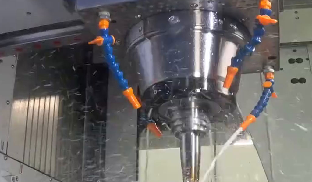
Numerical Control (NC) machine tools are pivotal in modern manufacturing, enabling precise and automated machining processes across industries such as aerospace, automotive, and medical device production. Among the various configurations, 3-axis NC machine tools are widely used due to their balance of simplicity, versatility, and precision. These machines operate by controlling the motion of a tool or workpiece along three orthogonal axes, typically denoted as X, Y, and Z. The kinematic modelling of such machines is essential for understanding and optimizing their performance in tasks requiring linear and circular interpolation, which are fundamental techniques for generating complex tool paths.

Kinematic modelling involves the mathematical representation of the machine’s motion, accounting for the relationships between the control inputs, axis movements, and the resulting tool path. Linear interpolation enables the tool to move in straight lines between programmed points, while circular interpolation allows the tool to follow circular or arc-shaped paths, critical for machining curved surfaces or contours. This article provides a comprehensive exploration of the kinematic modelling of 3-axis NC machine tools, focusing on the principles, mathematical frameworks, and practical considerations for linear and circular interpolation. It includes detailed discussions of coordinate systems, motion control algorithms, error analysis, and performance optimization, supplemented by comparative tables to elucidate key concepts.

Fundamentals of 3-Axis NC Machine Tools

Overview of 3-Axis NC Machine Tools

A 3-axis NC machine tool consists of a mechanical structure that allows motion along three linear axes: X (horizontal, left-right), Y (horizontal, front-back), and Z (vertical, up-down). These axes are typically driven by servo motors controlled by a computer numerical control (CNC) system, which interprets programmed instructions (e.g., G-code) to coordinate the motion of the tool or workpiece. The machine’s kinematic chain includes components such as lead screws, ball screws, linear guides, and motors, which translate electrical signals into precise mechanical movements.

The primary advantage of 3-axis machines lies in their ability to machine complex geometries with relatively simple setups compared to multi-axis systems (e.g., 5-axis machines). They are commonly used in milling, drilling, and turning operations, where the tool or workpiece moves in a Cartesian coordinate system to achieve the desired shape. Understanding the kinematics of these machines requires analyzing the relationships between the control system, axis dynamics, and the resulting tool path accuracy.

Coordinate Systems in 3-Axis NC Machines

The kinematic modelling of a 3-axis NC machine begins with defining its coordinate systems. The machine operates in a Cartesian coordinate system, where each axis corresponds to a linear degree of freedom. The coordinate system is typically divided into:

• Machine Coordinate System (MCS): The fixed reference frame of the machine, defined by the physical limits of the axes. The origin is usually set at a reference point (e.g., the home position).

• Workpiece Coordinate System (WCS): The coordinate system aligned with the workpiece, which may be offset from the MCS to account for fixturing or part positioning.

• Tool Coordinate System (TCS): The coordinate system associated with the tool tip, which moves relative to the MCS and WCS during machining.

The transformation between these coordinate systems is critical for accurate tool path generation. For example, the position of the tool tip in the WCS can be expressed as:

[ \mathbf{P}{WCS} = \mathbf{P}{MCS} + \mathbf{T}_{offset} ]

where (\mathbf{P}{WCS}) is the tool position in the workpiece coordinate system, (\mathbf{P}{MCS}) is the tool position in the machine coordinate system, and (\mathbf{T}_{offset}) is the offset vector accounting for the workpiece’s position relative to the machine’s origin.

Role of Interpolation in NC Machining

Interpolation is the process of generating intermediate points along a tool path to ensure smooth and accurate motion between programmed positions. In 3-axis NC machines, the two primary interpolation methods are:

• Linear Interpolation: The tool moves in a straight line between two points by coordinating the simultaneous motion of the X, Y, and/or Z axes.

• Circular Interpolation: The tool follows a circular or arc-shaped path, typically in the XY, XZ, or YZ plane, defined by a center point, radius, and angular span.

Interpolation algorithms are implemented in the CNC controller, which calculates the required axis velocities and positions to achieve the desired path while maintaining the programmed feed rate and accuracy. The kinematic model must account for the machine’s dynamic response, including acceleration, deceleration, and potential sources of error such as backlash or thermal expansion.

Kinematic Modelling Principles

Kinematic Chain of a 3-Axis NC Machine

The kinematic chain of a 3-axis NC machine describes the sequence of components and joints that translate control inputs into tool motion. A typical kinematic chain includes:

1. Servo Motors: Provide rotational motion to drive the axes.

2. Transmission Elements: Convert rotational motion into linear motion (e.g., ball screws or rack-and-pinion systems).

3. Linear Guides: Ensure precise linear motion along each axis.

4. Tool or Workpiece Holder: Positions the tool or workpiece relative to the machine frame.

The kinematic model represents the position of the tool tip as a function of the axis positions. For a 3-axis machine, the tool position in the MCS can be expressed as:

[ \mathbf{P}_{tool} = [x, y, z]^T ]

where (x), (y), and (z) are the positions of the X, Y, and Z axes, respectively. The simplicity of this model assumes ideal conditions, such as perfect alignment and no mechanical errors. In practice, the model must account for non-idealities, such as axis misalignment or servo lag.

Forward and Inverse Kinematics

Kinematic modelling involves both forward and inverse kinematics:

• Forward Kinematics: Determines the tool’s position and orientation given the axis positions. For a 3-axis machine, this is straightforward, as the tool position is directly equal to the axis positions (assuming no offsets or errors).

• Inverse Kinematics: Calculates the required axis positions to achieve a desired tool position. In 3-axis machines, inverse kinematics is trivial because the axes are orthogonal, and the tool position directly corresponds to the axis coordinates.

However, practical considerations, such as tool length compensation or workpiece offsets, may introduce complexity. For example, if the tool length is (L), the effective tool tip position in the Z-axis is adjusted as:

[ z_{effective} = z - L ]

Dynamic Considerations

While kinematic models focus on the geometric relationships of motion, dynamic factors such as acceleration, jerk, and inertia affect the machine’s performance. The CNC controller must ensure that axis movements are synchronized to maintain the desired tool path, especially during high-speed machining. The dynamic model can be represented by the equations of motion for each axis:

[ F_i = m_i \ddot{x}_i + c_i \dot{x}_i + k_i x_i ]

where (F_i) is the force applied to axis (i), (m_i) is the mass, (c_i) is the damping coefficient, (k_i) is the stiffness, and (x_i), (\dot{x}_i), (\ddot{x}_i) are the position, velocity, and acceleration, respectively. These equations are solved numerically by the CNC controller to generate smooth motion profiles.

Linear Interpolation

Principles of Linear Interpolation

Linear interpolation involves moving the tool in a straight line from a starting point (\mathbf{P}_1 = [x_1, y_1, z_1]) to an ending point (\mathbf{P}_2 = [x_2, y_2, z_2]) at a specified feed rate (F). The tool path is parameterized by a scalar (t \in [0, 1]), where:

[ \mathbf{P}(t) = \mathbf{P}_1 + t (\mathbf{P}_2 - \mathbf{P}_1) ]

The components of the tool position are:

[ x(t) = x_1 + t (x_2 - x_1) ] [ y(t) = y_1 + t (y_2 - y_1) ] [ z(t) = z_1 + t (z_2 - z_1) ]

The feed rate determines the speed of motion along the path. The total distance (S) between the points is:

[ S = \sqrt{(x_2 - x_1)^2 + (y_2 - y_1)^2 + (z_2 - z_1)^2} ]

The time (T) to traverse the path is:

[ T = \frac{S}{F} ]

The CNC controller calculates the required velocities for each axis ((\dot{x}), (\dot{y}), (\dot{z})) to ensure the tool moves at the specified feed rate while maintaining the linear path.

Implementation in CNC Systems

In a CNC system, linear interpolation is typically programmed using G-code commands, such as:

G01 Xx2 Yy2 Zz2 Ff

where (G01) specifies linear interpolation, (Xx2 Yy2 Zz2) defines the target position, and (Ff) specifies the feed rate in units per minute (e.g., mm/min). The controller discretizes the path into small segments, calculating the axis positions at each time step to achieve smooth motion.

The interpolation algorithm must account for the machine’s dynamic constraints, such as maximum axis velocities and accelerations. For example, if the X-axis has a maximum velocity (V_{max,X}), the controller ensures that:

[ |\dot{x}| \leq V_{max,X} ]

If the required velocity exceeds the limit, the controller scales down the feed rate to maintain synchronization across all axes.

Error Sources in Linear Interpolation

Several factors can introduce errors in linear interpolation:

1. Quantization Error: The CNC controller operates with finite resolution, leading to small deviations in the calculated positions.

2. Axis Misalignment: Non-orthogonality between axes can cause the tool path to deviate from a straight line.

3. Backlash: Mechanical play in the transmission system can result in positioning errors.

4. Servo Lag: Delays in the servo system’s response can cause the tool to lag behind the commanded position.

To mitigate these errors, modern CNC systems employ techniques such as backlash compensation, feedforward control, and high-resolution encoders.

Table 1: Comparison of Linear Interpolation Parameters

Circular Interpolation

Principles of Circular Interpolation

Circular interpolation enables the tool to follow a circular arc, typically in one of the principal planes (XY, XZ, or YZ). The arc is defined by:

• Start Point: The initial position of the tool, e.g., (\mathbf{P}_1 = [x_1, y_1, z_1]).

• End Point: The final position, e.g., (\mathbf{P}_2 = [x_2, y_2, z_2]).

• Center Point: The center of the arc, e.g., (\mathbf{C} = [x_c, y_c, z_c]).

• Radius ((R)): The radius of the arc.

• Direction: Clockwise (G02) or counterclockwise (G03).

For an arc in the XY plane, the tool position is parameterized by the angular position (\theta):

[ x(\theta) = x_c + R \cos(\theta) ] [ y(\theta) = y_c + R \sin(\theta) ] [ z(\theta) = z_1 \text{ (constant for XY plane)} ]

The angular velocity (\omega) is determined by the feed rate (F) and radius (R):

[ \omega = \frac{F}{R} ]

The time to traverse an arc of angular span (\Delta\theta) is:

[ T = \frac{R \Delta\theta}{F} ]

Implementation in CNC Systems

Circular interpolation is programmed using G-code commands, such as:

G02 Xx2 Yy2 Ixi Jyj Ff

where (G02) specifies clockwise circular interpolation, (Xx2 Yy2) is the end point, (Ixi Jyj) defines the center point relative to the start point (i.e., (x_c - x_1), (y_c - y_1)), and (Ff) is the feed rate. For counterclockwise motion, (G03) is used.

The CNC controller calculates the intermediate points along the arc by discretizing the angular parameter (\theta). The step size (\Delta\theta) is chosen to balance accuracy and computational efficiency. The axis velocities are:

[ \dot{x} = -R \sin(\theta) \omega ] [ \dot{y} = R \cos(\theta) \omega ]

Challenges in Circular Interpolation

Circular interpolation is more complex than linear interpolation due to the nonlinear nature of the tool path. Key challenges include:

1. Chordal Error: The discretization of the arc into linear segments introduces a chordal error, where the tool path approximates the arc with straight lines. The error is proportional to the step size and inversely proportional to the radius.

2. Radius Mismatch: Small discrepancies in the programmed start and end points can result in a radius mismatch, causing the controller to adjust the path or generate an error.

3. Dynamic Constraints: The rapid changes in axis velocities required to follow a circular path can exceed the machine’s acceleration or jerk limits, leading to path deviations.

Modern CNC systems mitigate these issues using adaptive interpolation algorithms, which adjust the step size based on the arc’s curvature and the machine’s dynamic capabilities.

Table 2: Comparison of Circular Interpolation Parameters

Advanced Kinematic Modelling Techniques

Parametric Path Representation

To improve the flexibility and accuracy of tool path generation, kinematic models often use parametric representations. For linear interpolation, the path is parameterized by a single parameter (t). For circular interpolation, the angular parameter (\theta) is used. More complex paths, such as splines or Bezier curves, may be approximated using linear and circular segments in 3-axis machines.

A general parametric path in 3D space can be expressed as:

[ \mathbf{P}(u) = [x(u), y(u), z(u)] ]

where (u) is the parameter (e.g., (u = t) for linear interpolation or (u = \theta) for circular interpolation). The CNC controller computes the derivatives (\dot{x}(u)), (\dot{y}(u)), (\dot{z}(u)) to determine the axis velocities.

Look-Ahead Algorithms

Modern CNC systems employ look-ahead algorithms to optimize tool path execution. These algorithms analyze upcoming G-code blocks to anticipate changes in direction, feed rate, or interpolation type. For example, when transitioning from linear to circular interpolation, the controller may reduce the feed rate to avoid exceeding acceleration limits at the junction point.

The look-ahead algorithm solves an optimization problem to minimize machining time while satisfying constraints such as:

[ |\ddot{x}i| \leq a{max,i}, \quad |\dddot{x}i| \leq j{max,i} ]

where (a_{max,i}) and (j_{max,i}) are the maximum acceleration and jerk for axis (i).

Error Compensation Techniques

To enhance accuracy, kinematic models incorporate error compensation techniques, such as:

• Geometric Error Compensation: Corrects for axis misalignment or non-orthogonality using calibration data.

• Thermal Compensation: Adjusts for thermal expansion of machine components based on temperature measurements.

• Backlash Compensation: Accounts for mechanical play by adding corrective movements to the axis commands.

These techniques require accurate measurement of the machine’s error sources, typically using laser interferometry or ballbar testing.

Performance Optimization

Feed Rate Optimization

Optimizing the feed rate is critical for balancing machining speed and accuracy. Adaptive feed rate algorithms adjust the feed rate based on the path curvature, machine dynamics, and material properties. For example, in circular interpolation, the feed rate may be reduced for small-radius arcs to maintain accuracy.

The optimal feed rate can be determined by solving:

[ F_{opt} = \min(F_{max}, F_{dynamic}, F_{accuracy}) ]

where (F_{max}) is the machine’s maximum feed rate, (F_{dynamic}) is the feed rate limited by axis dynamics, and (F_{accuracy}) is the feed rate constrained by error tolerances.

Tool Path Smoothing

Tool path smoothing techniques reduce abrupt changes in direction or velocity, minimizing vibrations and improving surface finish. Common methods include:

• Corner Rounding: Inserts small arcs at sharp corners to smooth transitions between linear segments.

• Spline Interpolation: Approximates the tool path with smooth curves, such as cubic splines, to reduce jerk.

These techniques require modifications to the kinematic model to account for the smoothed paths.

Table 3: Comparison of Optimization Techniques

Practical Applications

Case Study: Milling a Complex Contour

Consider a milling operation to create a complex contour on a workpiece, requiring both linear and circular interpolation. The tool path consists of straight segments for the outer profile and circular arcs for rounded corners. The kinematic model ensures that the tool follows the path accurately by coordinating the X and Y axes for circular interpolation and all three axes for linear segments.

The G-code for a sample contour might include:

G01 X10 Y10 F500 ; Linear move to (10, 10)
G02 X20 Y20 I5 J0 F500 ; Clockwise arc to (20, 20) with center offset (5, 0)
G01 X30 Y20 F500 ; Linear move to (30, 20)

The CNC controller uses the kinematic model to calculate the axis velocities and ensure smooth transitions between segments.

Industrial Applications

3-axis NC machines are used in various applications, including:

• Aerospace: Machining lightweight components with complex geometries, such as turbine blades.

• Automotive: Producing molds and dies for body panels.

• Medical Devices: Fabricating precision components, such as orthopedic implants.

The kinematic model is critical for ensuring that these applications meet stringent tolerances.

Future Trends in Kinematic Modelling

Integration with Digital Twins

Digital twins—virtual representations of physical machines—are increasingly used to enhance kinematic modelling. By simulating the machine’s behavior in real time, digital twins enable predictive maintenance, error detection, and optimization of tool paths. The kinematic model forms the core of the digital twin, providing the mathematical foundation for simulating motion.

Machine Learning for Error Compensation

Machine learning algorithms are being applied to kinematic modelling to predict and compensate for errors. For example, neural networks can learn the relationship between machining conditions (e.g., temperature, feed rate) and errors, enabling real-time adjustments to the tool path.

Table 4: Future Trends in Kinematic Modelling

Conclusion

The kinematic modelling of 3-axis NC machine tools is a cornerstone of modern manufacturing, enabling precise control of tool paths in linear and circular interpolation. By understanding the principles of coordinate systems, interpolation algorithms, and error compensation, engineers can optimize machine performance for a wide range of applications. The integration of advanced techniques, such as look-ahead algorithms, digital twins, and machine learning, promises to further enhance the capabilities of 3-axis NC machines, ensuring their continued relevance in precision manufacturing.

Reprint Statement: If there are no special instructions, all articles on this site are original. Please indicate the source for reprinting:https://www.cncmachiningptj.com/，thanks！

PTJ® provides a full range of Custom Precision cnc machining china services.ISO 9001:2015 &AS-9100 certified. 3, 4 and 5-axis rapid precision CNC machining services including milling, turning to customer specifications,Capable of metal & plastic machined parts with +/-0.005 mm tolerance.Secondary services include CNC and conventional grinding, drilling,die casting,sheet metal and stamping.Providing prototypes, full production runs, technical support and full inspection.Serves the automotive, aerospace, mold&fixture,led lighting,medical,bicycle, and consumer electronics industries. On-time delivery.Tell us a little about your project's budget and expected delivery time. We will strategize with you to provide the most cost-effective services to help you reach your target,Welcome to Contact us ( sales@pintejin.com ) directly for your new project.